Pandas vs PySpark: How to Choose the Right Tool for Your Data Ingestion Pipeline

3 weeks ago

12 9 minutes read

Introduction

Moving data from source to sink is the first technical step in a data pipeline. This process, called data ingestion, can be deceptively complex. Should you use a simple library like Pandas or a more advance library like PySpark? In this article, you learn how to choose the right tool for your data ingestion pipeline.

I will walk through a hands-on process of ingesting a CSV file into a Google Cloud Storage with both Pandas and PySpark. This means out project stack is:

Language: Python (3.8 or later installed.)

Core Libraries: Pandas, PySpark

Data Lake: Google Cloud Storage (GCS)

Prerequisites:

A beginner knowledge in python is essential but not compulsory as I will be explaining every code snippet. You will need a Google Cloud Storage (GCP) account with billing enabled. Don’t worry, you won’t be charged as long as you delete the resources you created.

Overview of Pandas and PySpark

Before we write any code, let’s understand the fundamental difference. Choosing between Pandas and PySpark is a classic data engineering dilemma that boils down to a single word: scale.

Choose Pandas for single-machine processing. It’s perfect for smaller datasets (gigs of data, not terabytes) that can comfortably fit into your computer’s memory (RAM). It is incredibly fast and intuitive for exploration, cleaning, and ingesting data for proof-of-concept projects or smaller applications.

Choose PySpark for distributed processing. When your data is too large to fit into the memory of a single machine—the “Big Data” problem—you need PySpark. It’s the Python API for Apache Spark, a powerful engine that distributes data and computations across a cluster of multiple computers, allowing you to process massive datasets efficiently.

For our project today, we’ll start with a small CSV file where Pandas excels. Then, we’ll show how the same logic applies in PySpark, making it clear how you would scale up when needed.

This is the heart of our project. We will build a simple pipeline to ingest a public dataset into our Google Cloud Storage data lake, but first, we need to set up the destination.

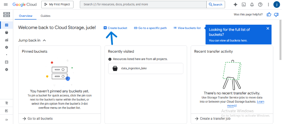
Set Up Your Google Cloud Storage Bucket

Our Google Cloud Storage bucket will act as our data lake, a central place to store raw data.

Navigate to the Google Cloud Console and sign in.

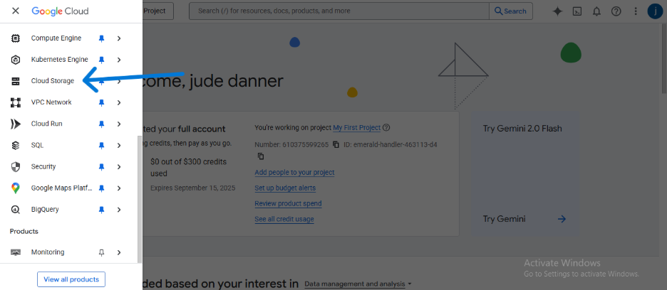
Using the main navigation menu, go to Cloud Storage > Buckets.

Click CREATE.

Give your bucket a globally unique name (e.g., dekings-raw-data-lake-123).

Choose the Standard storage class and Uniform access control.

Select a Location for your bucket (e.g., us-central1 (Iowa)).

Click CREATE.

Create and Secure a Service Account Key

To allow our Python script to securely access and write files to our Google Cloud bucket, we need to create a Service Account. Think of this as a special type of user account designed for applications, not people.

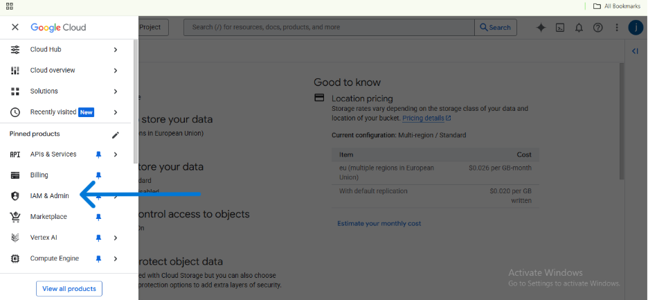
In the Google Cloud Console, open the main navigation menu (the “hamburger” icon ☰) and go to IAM & Admin > Service Accounts.

At the top, click + CREATE SERVICE ACCOUNT.

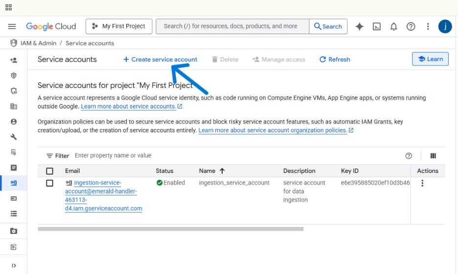
Give your service account a clear name, like gcs-ingestion-service, and add a brief description. The Service account ID will be created for you automatically. Click CREATE AND CONTINUE.

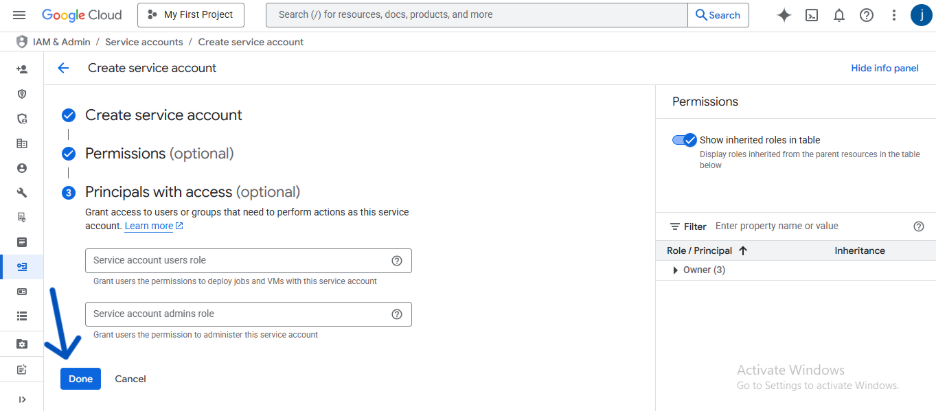
Next, we need to give the account permission to do its job. Click the Select a role dropdown menu and search for Storage Object Admin(ensure to give the right access to the right person). Select it. This role grants our script the necessary permissions to create, read, and delete files in our GCS buckets. Click CONTINUE.

You can skip the last optional step (“Grant users access to this service account”). Click DONE.

You’re now back on the Service Accounts page. Find the account you just created and click on its email address in the Principal column.

Navigate to the KEYS tab. Click ADD KEY > Create new key.

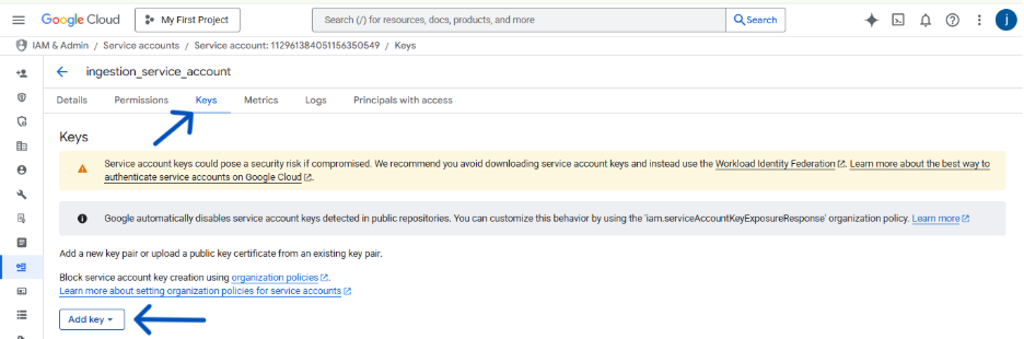
Choose JSON as the key type and click CREATE.

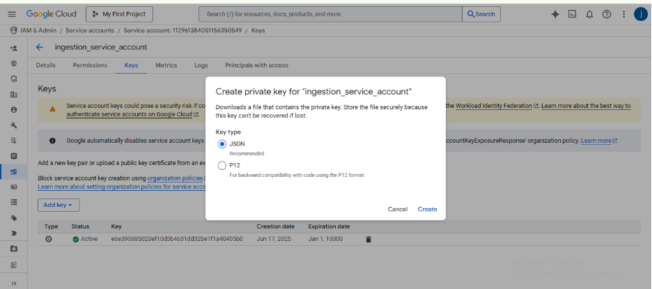
Your browser will immediately download a JSON file. This file contains the private credentials for your service account.

⚠️ Security Warning: Treat this downloaded JSON file like a password. Never commit it to a public Git repository. Anyone who has this file can access your Google Cloud Storage. Store it in a secure location on your computer.

Now that our GCS data lake and service account are ready, it’s time to write the Python scripts to perform the ingestion. We’ll start with Pandas and then show how to perform the same task with PySpark.

Data Ingestion with Pandas

We’ll begin with Pandas because it’s perfect for the kind of smaller, single-file data ingestion tasks you’ll often encounter. Our goal is to read a CSV file from a public URL and write it as a Parquet file into our GCS bucket.

Setup and Dependencies

First, you need to install the necessary libraries. gcsfs allows Pandas to communicate directly with Google Cloud Storage.

pip install pandas google-cloud-storage gcsfs

Next, we need to tell our script how to authenticate. Instead of putting the path to your service account key in the code, we’ll set an environment variable. This is a critical security best practice.

On macOS/Linux:

export GOOGLE_APPLICATION_CREDENTIALS="/path/to/your/keyfile.json"

On Windows (Command Prompt):

set GOOGLE_APPLICATION_CREDENTIALS="C:\path\to\your\keyfile.json"

Pandas Ingestion Script

Now, create a Python file named ingest_with_pandas.py and add the following code. It’s a complete, runnable script.

ingest_with_pandas.py — file

import pandas as pd import os 

def ingest_data_with_pandas():  

   """ Reads a public parquet file, converts it to a DataFrame, and uploads it as a Parquet file to Google Cloud Storage. 

   """ 

   # 1. Define variables 

   # Public URL of the dataset (NYC Taxi Data for Jan 2024) 

   # Note: We use a smaller, specific file for this example. 
 
   SERVICE_KEY_PATH = os.getenv('GOOGLE_APPLICATION_CREDENTIALS') 
 
   source_url = "https://d37ci6vzurychx.cloudfront.net/trip-data/yellow_tripdata_2024-01.parquet" 
 
   # Your GCS bucket name 
   bucket_name = "data_ingestion_lake4" # <--- Replace with your bucket name! 
 
   # Desired name for the output file in GCS 
   destination_file_name = "ny_taxi_data_2024_01.parquet" 
 
   print(f"--> Reading Parquet file from {source_url}...") 
 
   # 2. Load data into a Pandas DataFrame 

   # Pandas can read directly from a URL 
   df = pd.read_parquet(source_url) 
   print(f"    Success! DataFrame created with {len(df)} rows.") 
   print(df.head())  # Display the first few rows of the DataFrame 
 
   # 3. Construct the GCS path and write the file 
   # The 'gs://' prefix tells pandas to use the gcsfs library 
   gcs_path = f"gs://{bucket_name}/{destination_file_name}" 
 
   print(f"--> Writing DataFrame to {gcs_path}...") 
 
   # Using 'to_parquet' to write to GCS. 
   # The gcsfs library uses your GOOGLE_APPLICATION_CREDENTIALS 
   # environment variable automatically for authentication. 
   df.to_parquet(gcs_path, index=False) 
 
 
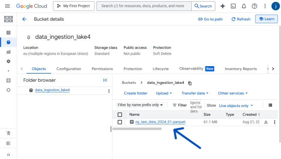
   print(f" Success! {len(df)} rows have been uploaded to your bucket.") 
  

ingest_data_with_pandas()

Run this script from your terminal. It will download the data, process it in memory, and upload the result to your GCS bucket. Just like that, you’ve performed a data ingestion task with Pandas!

Daat Ingestion with PySpark. Scale Up with PySpark

Now, imagine that taxi data wasn’t for one month, but for ten years—far too big to fit in your computer’s memory. This is where Pandas breaks down and PySpark shines.

Let’s perform the exact same task using PySpark to see how the approach differs.

Setup and Dependencies

You’ll need to install pyspark.

pip install pyspark

Create a new file called ingest_with_pyspark.py in your project folder. Notice how we first configure a SparkSession to communicate with GCS before we do any data processing.


from pyspark.sql import SparkSession 

import pandas as pd 

import os 

def ingest_data_with_pyspark():  

   """Initializes a SparkSession with GCS connector, reads a public Parquet file using pandas, converts it to Spark DataFrame, and writes it back to a GCS bucket. 

   """  

   print("--> Initializing Spark Session...") 

   spark = SparkSession.builder \ 
       .appName('GCS_Ingestion_PySpark') \ 
       .config("spark.jars", "https://storage.googleapis.com/hadoop-lib/gcs/gcs-connector-hadoop3-latest.jar") \ 
       .config("spark.sql.execution.arrow.pyspark.enabled", "true") \ 
       .getOrCreate() 
   print("    Success! Spark Session created.") 
 
   # 1. Define variables 
   SERVICE_KEY_PATH = os.getenv('GOOGLE_APPLICATION_CREDENTIALS') 
   source_url = "https://d37ci6vzurychx.cloudfront.net/trip-data/yellow_tripdata_2024-01.parquet" 
   bucket_name = "ingestion_delta_lake2" 
   destination_file_name = "ny_taxi_data_pyspark_2024_01" 
 
   print(f"--> Reading Parquet file from {source_url} using pandas...") 
   # 2. Load data with pandas first, then limit to first 10,000 rows 
   pdf = pd.read_parquet(source_url).head(10000) 
   print(f"    Success! pandas DataFrame created with {len(pdf)} rows.") 
 
   # 3. Convert pandas DataFrame to Spark DataFrame using pyarrow 
   # Spark will automatically use pyarrow with the configuration set above 
   df = spark.createDataFrame(pdf) 
   print(f"    Converted to Spark DataFrame with {df.count()} rows.") 
   df.printSchema() 
 
   # 4. Construct the GCS path and write the file 
   gcs_path = f"gs://{bucket_name}/{destination_file_name}" 
   print(f"--> Writing Spark DataFrame to {gcs_path}...") 
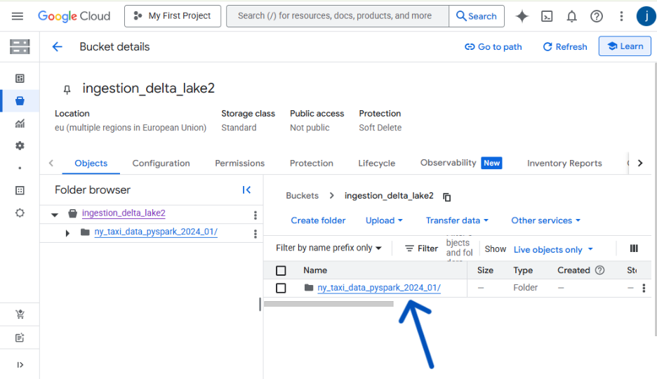
   df.write.mode('overwrite').parquet(gcs_path) 
   print(f"    Success! Data uploaded to your bucket.") 
 
   spark.stop() 
  

   if name == 'main': ingest_data_with_pyspark()

Before we continue, let me take a little time to breakdown what happens with parquet files.

The “Why”: Parallelism in Action 🏃‍♂️💨

PySpark creates multiple smaller files because it’s designed for parallel processing. Think of it like a team of cashiers at a supermarket.

Instead of one cashier scanning every single item (the Pandas approach), Spark acts like a manager who splits your shopping cart (the DataFrame) among several cashiers (worker tasks).

Each cashier scans their portion of the items simultaneously and puts them in their own bag (a Parquet file). This is much faster than waiting for one person to do all the work.

The number of small files created usually corresponds to the number of partitions your data was split into for processing.

The “How”: Treat the Directory as the Dataset 📂

The key takeaway is that you should almost never interact with the individual part-*.parquet files directly. Instead, you always point your tools to the main output directory.

Modern data tools like Spark and Pandas are built to understand this structure. When you provide the path to the parent folder, they automatically discover all the Parquet files within it and read them as a single, unified table.

You just point spark.read.parquet() to the main directory you wrote to.

The “Proof”: The _SUCCESS File ✅

So, how do you know the process finished and all the small files are present? Spark provides a simple, elegant solution: the _SUCCESS file.

When a Spark write job completes without any errors, it creates an empty file named _SUCCESS in the output directory. The presence of this file is a universal signal that the dataset is complete, correct, and ready to be used by downstream processes. If the job fails for any reason, this file will not be created.

In automated data pipelines, a common pattern is to use a sensor that waits for the _SUCCESS file to appear before kicking off the next task, ensuring you never work with incomplete data

With these two scripts, you now have a direct, hands-on comparison of how each tool accomplishes the same goal, setting the stage for our final analysis.

The Verdict: Making the Right Choice for Your Pipeline

Choosing between Pandas and PySpark for data ingestion isn’t about which tool is “better”—it’s about selecting the right tool for the scale of the job.

Here’s a summary of the key differences:

Feature	Pandas	PySpark
Processing	Single machine (uses one core at a time)	Distributed (uses multiple machines/cores)
Data Size	Small to medium (limited by local RAM)	Large (Terabytes/Petabytes; scales horizontally)
Performance	Faster for small datasets	Faster for massive datasets due to parallelism
Learning Curve	Easy, intuitive Python syntax	Steeper; requires understanding distributed concepts
Debugging	Straightforward, immediate feedback	More complex due to distributed execution
Use Case	Local analysis, POCs, small ETL jobs	Production-grade ETL, Big Data processing

When to Choose Pandas 🐼

Size: Your data fits comfortably in your machine’s memory (typically a few gigabytes).

Simplicity: You need to get the job done quickly with minimal setup and simple syntax.

Environment: You are working locally or on a single server.

Use Case: Ideal for initial data exploration, prototyping, or small-scale ingestion tasks.

When to Choose PySpark 🔥

Scale: Your data is too large to fit into a single machine’s memory.

Performance: You need parallelism to process large volumes of data quickly.

Environment: You are working in a distributed environment (e.g., Databricks, AWS EMR, or a Hadoop cluster).

Use Case: Ideal for building scalable, production-grade ETL pipelines.

Conclusion and Next Steps

In this article, we successfully built two ingestion pipelines to move data into Google Cloud Storage: one using the simplicity of Pandas and another using the scalable power of PySpark.

The key takeaway is that scale dictates the tool. Pandas is excellent for speed and simplicity when your data fits in memory, while PySpark is essential when you need distributed processing power for big data.

🚀 Next Steps

Ready to build on what you’ve learned? Here are a few ways to extend this project:

Error Handling: Add try…except blocks to both scripts to handle potential network issues or authentication errors gracefully.

Data Transformation: Before writing the data to GCS, try adding a simple transformation.

Pandas: Use .rename() or .drop() to clean up column names or remove unnecessary data.

PySpark: Use .withColumnRenamed() or .select() to achieve the same result in a distributed manner.

Explore Spark Configuration: Dive deeper into the SparkSession configuration. Try adjusting the number of partitions when writing the Parquet files using df.repartition(N).write… and see how it affects the output.

Mastering both Pandas and PySpark ensures you always have the right tool in your data engineering toolkit, no matter the size of the challenge.